

Your customer acquisition cost is judged against the wrong number
About this series. Which customers are worth paying for? We are working through customer lifetime value on two years of real order history from a UK online retailer (UCI Online Retail II, an open dataset), because it is the question every acquisition budget quietly depends on. Part 1 asks whether the number campaigns are judged on is the right one. Parts 2 to 4 cover predicting lifetime value, handing that prediction to your ad platform, and when the platform's own predictions are enough.
The standard way to judge an acquisition campaign is revenue from the first order, divided by what it cost to get it. It is the number the ad platform reports, so it is the number that gets used. The question is how good it is at telling you who you just acquired. We took two years of orders from a real retailer — 5,852 identified customers, every invoice — and checked.
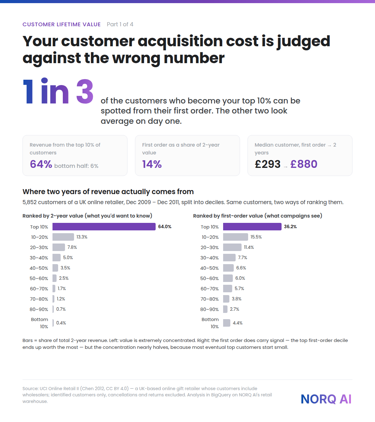
64%of two-year revenue came from the top 10% of customers; 6% from the bottom half
14%of a customer's two-year value was in their first order
1 in 3of the eventual top-10% customers were visible from their first order
Value is concentrated — more than most plans assume
Rank customers by what they spent over the two years and the top tenth produced 64% of all revenue. The top fifth produced 77%. The bottom half, 6%. This is a gift retailer with some wholesale buyers, so the concentration is at the sharp end of what a consumer shop would see, but the shape — a small group carrying most of the value — is the normal one, and it changes what "a good customer" means. Average customer value is a number almost no customer has: the mean two-year value was £2,969; the median was £880.
The first order is a small part of the story
Across all customers, the first order was 14% of what they went on to spend. The median customer's first order was £293; the median customer's two-year value was £880. Seventy-two percent of customers ordered more than once. A campaign judged on first-order revenue is being judged on roughly a seventh of what it actually bought.
That would be fine if the first order at least ranked customers correctly — if the big first orders were the big customers. The right-hand chart shows they partly are: the top decile by first order did end up worth the most, with 36% of revenue. The first order carries real signal. But the concentration nearly halves compared with the truth on the left, because most eventual top customers did not announce themselves.
One in three
The cleanest way to put it: take the 586 customers who ended up in the top 10% by two-year value, and ask how many were in the top 10% by first-order value. The answer is 196 — one in three. The other two looked average on day one, and an acquisition process optimising for first-order revenue would have treated them accordingly: bid less for people like them, spend less to retain them, report them as mediocre.
| Customers ranked by… | Top decile's share of revenue | Avg. orders in top decile | Repeat rate in top decile |
|---|---|---|---|
| Two-year value (the truth) | 64.0% | 26.8 | 99% |
| First-order value (what campaigns see) | 36.2% | 10.0 | 80% |
What this means for your shop
The number used to judge acquisition — first-order ROAS — is not wrong, it is early. It is measured before most of a customer's value exists, and it identifies a minority of the customers that matter. The consequence is not academic: bidding algorithms optimise for whatever value they are given. Give them first-order revenue and they will find you customers who place large first orders, which is a different population from customers who stay.
Under the hood — for the technically curious
The source is a static Excel workbook, loaded once into BigQuery and declared as a source
to Dataform. Staging removes cancellations (invoices prefixed C), returns
(negative quantities), zero prices, non-product stock codes (postage, manual adjustments,
bank charges) and exact duplicate rows — about 20% of the raw lines. Unidentified
customers (23% of lines, mostly guest checkouts) are kept for revenue totals and excluded
from customer-level analysis. From there: an order-grain fact and a customer dimension
with first/last order, order count, revenue and first-order revenue, plus the
frequency/recency/age inputs that part 2's BG/NBD model needs.
The concentration numbers are one query on that dimension:
WITH c AS (
  SELECT customer_id, revenue_gbp, first_order_revenue_gbp,
    NTILE(10) OVER (ORDER BY revenue_gbp DESC)             AS value_decile,
    NTILE(10) OVER (ORDER BY first_order_revenue_gbp DESC) AS first_order_decile
  FROM dim_uci_customers
),
tot AS (SELECT SUM(revenue_gbp) AS total FROM c)
SELECT value_decile,
  COUNT(*)                                   AS customers,
  ROUND(SUM(revenue_gbp) / t.total * 100, 1) AS pct_of_revenue
FROM c CROSS JOIN tot t
GROUP BY value_decile, t.total
ORDER BY value_decile
And the one-in-three:
WITH c AS (
  SELECT
    PERCENT_RANK() OVER (ORDER BY revenue_gbp DESC)             < 0.1 AS top_by_lifetime,
    PERCENT_RANK() OVER (ORDER BY first_order_revenue_gbp DESC) < 0.1 AS top_by_first_order
  FROM dim_uci_customers
)
SELECT
  COUNTIF(top_by_lifetime)                        AS top_customers,
  COUNTIF(top_by_lifetime AND top_by_first_order) AS visible_from_first_order
FROM c
The same two queries run unchanged on any order table with a customer key, an order date and a revenue column — which is the point. This is not a model. It is a question your warehouse can already answer.
Data and licence
Chen, D. (2012). Online Retail II [Dataset]. UCI Machine Learning Repository, doi:10.24432/C5CG6D, licensed CC BY 4.0. All transactions of a UK-based, non-store online retailer of unique all-occasion giftware, 1 December 2009 to 9 December 2011; many customers are wholesalers. 1.07 million lines, 53,600 invoices, 5,942 identified customers before cleansing.
Next in the series: predicting a customer's value from their first weeks (BG/NBD and Gamma-Gamma, in plain terms), then teaching Google Ads what a good customer is. Related: Your analytics data is lying to your recommender, part 1 of our recommendation-systems series.
Start Your Data Transformation Journey
Discover practical, scalable solutions tailored to your business priorities.